

Bε-Tree – B-Epsilon Tree – Beta-Epsilon Tree – the Bε, B-Epsilon and Beta Epsilon tree terms apply to the same concept, a B-tree with buffers. We’ll call it the Bε tree and say it combines the write strength of LSM trees and the read strength of B-trees. The Bε tree is a modification of B-trees that support much higher write throughput. This is achieved by adding a buffer to each node in the tree so that you don’t need to travel all the way down the tree every time to find the desired value. When a buffer is full all its contents are pushed down to the next level in one batch.
A Bε-tree is composed of a start or root node and child nodes with data-storing leaf nodes below them. Bε-trees encode updates as messages that are inserted at the root of the tree. Bε-tree leaf nodes store key-value pairs. Internal Bε-tree node buffers store messages. Messages target a specific key and encode a mutation.
Here is a Bε-tree diagram from Carnegie Mellon University lecture notes:
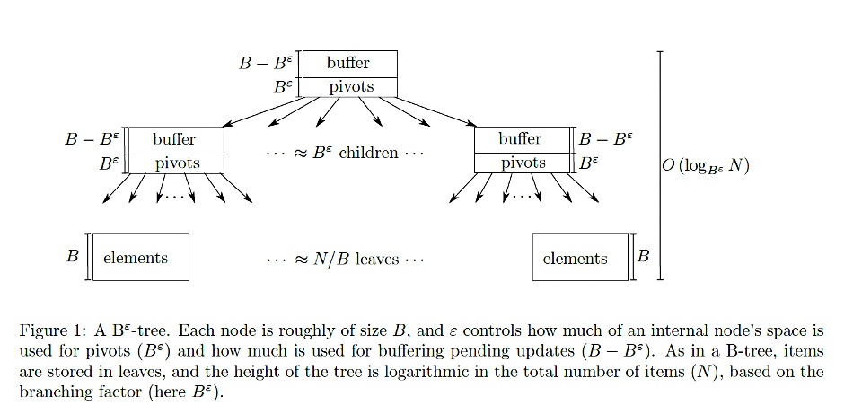
The lecture notes say the top node is the root node. Below that are child nodes with a layer of leaf nodes below them. A pivot is a key stored in an internal node of the Bε-tree that acts as a separator or boundary for directing searches to the appropriate child node. It determines the range of key values stored in the child nodes. For example, if a parent node has a pivot key ( k ), keys less than ( k ) are routed to the left child, and keys greater than or equal to ( k ) are routed to the right child.
Moving messages down the tree in batches is the key to the B”-tree’s insert performance. By storing newly-inserted messages in a buffer near the root, a B”-tree can avoid seeking all over the disk to put elements in their target locations. The B”-tree only moves messages to a subtree when enough messages have accumulated for that subtree to amortize the I/O cost. Although this involves rewriting the same data multiple times, this can improve performance for smaller, random insert.
Bε-trees delete items by inserting “tombstone messages” into the tree. These tombstone messages are flushed down the tree until they reach a leaf. When a tombstone message is flushed to a leaf, the Bε-tree discards both the deleted item and the tombstone message. Thus, a deleted item, or even entire leaf node, can continue to exist until a tombstone message reaches the leaf. Because deletes are encoded as messages, deletions are algorithmically very similar to insertions.
A high-performance Bε-tree should detect and optimize the case where a a large series of messages all go to one leaf. Suppose a series of keys are inserted that will completely fill one leaf. Rather than write these messages to an internal node, only to immediately rewrite them to each node on the path from root to leaf, these messages should flush directly to the leaf, along with any other pending messages for that leaf.
From an arXiv paper:
- Bε-trees, like B-trees, are trees of nodes of size B. All Bε-tree leaves are at the same height, all Bε-tree keys are stored in binary search tree order, and every Bε-tree node has (Bε) children. Bε-tree nodes maintain internal state so that these invariants can be maintained efficiently.
- Each Bε-tree node has a buffer in which messages can be stored. (Thus, a node can be read or written in a single IO.)
- To insert an item into a Bε-tree, place the item in the root node’s buffer. Then, recursively flush as follows: if the buffer of a node v is full, go through all B items in the buffer and determine which child they would be flushed to next. The child with the most such items is flushed to, moving every possible item to that child; recurse if the child now has B or more items.
- To query an item, traverse the root-to-leaf path p of the tree using the binary search tree ordering. The binary search tree ordering guarantees that the queried item is stored along this path. For each node v in p, determine if any of the B items in the buffer of v are the queried item.
Bε-tree searches are just as fast as B-trees. Bε-tree updates are orders-of-magnitude faster for inserts and updates due to their ability to batch small updates into large I/Os.
Note 1.
The Disk Access Machine (DAM) model [2] is a powerful tool for theoretically describing the cache efficiency of a data structure. In the DAM model there are three machine-dependent parameters:
- B, the size of a cache line;
- P, the number of disk accesses that can be performed in parallel;
- M ≫ PB, the size of the cache.
In a single IO, the data structure can read or write up to P sets of B contiguous elements to or from cache. The cost of any process under the DAM model is defined as the number of IOs required to complete the process.
A write-optimized data (WOD) structure handles inserts lazily: rather than traversing the data structure to put newly-inserted items directly in place, up to B items are accumulated and moved through the data structure in large IOs. Write-optimized data structures greatly improve insert performance in the DAM model. For example, if the cache size B is much larger than the height of the data structure, a write-optimized data structure requires o(1) IOs per insertion. This improvement in write cost comes at no asymptotic cost to query time.
LSM-trees, Bε-trees, and their variants are popular WODs that have been used to implement file systems, key-value stores, and other applications where cache efficiency is critical.
Note 2.
The efficiency of an index depends on how well it minimizes disk accesses. For example, a B-tree is designed to have a high fan-out (many keys per node) to reduce the height of the tree, thereby reducing the number of disk I/Os needed to locate a record.
In a B-tree, each node is typically the size of a disk block (or a multiple of it). This allows the tree to store many keys and pointers in a single node, reducing the number of disk accesses needed to traverse the tree.
For a search operation, the number of disk I/Os is proportional to the height of the B-tree, which is O(\log_B N), where ( B ) is the number of keys per node (related to block size) and ( N ) is the number of records. This logarithmic factor ensures efficient access even for very large datasets.


